noʜɈγԳ ʜɈiw ϱniʞɒmqɒM ɘviɈɔɒɿɘɈnI
nɒnɒʜƨɿɒϱnɒƧ
Interactive Mapmaking with Python
Sangarshanan
Data + Pandas ❤️
In [1]:
import pandas
df = pandas.read_csv('data/cities.csv')
df.head()
Out[1]:
Data with a location component 📍
Geometries
- Point (latitude, longitude)
- Polygon [point1, point2]
We can also have linestrings, multipolygons, circles etc
Enter GeoPandas

- Work with a Familiar interface (Dataframes), in this case Geodataframes
- Read/ write GIS data (Fiona) formats like shapefile, geojson, kml etc
- Perform spatial operations like merge/join/overlay etc (Shapely)
- Plot em on a map (Matplotlib)
Also a whole lot of other things !!!
Interested in more, https://github.com/jorisvandenbossche/geopandas-tutorial
In [2]:
df.head()
Out[2]:
In [3]:
import geopandas
# Converting latitude, longitude to geometry object
gdf = geopandas.GeoDataFrame(
    df, geometry=geopandas.points_from_xy(df.longitude, df.latitude))
# setting the projection
gdf.crs = 'epsg:4326'
gdf.head()
Out[3]:
How do I plot em ?
With geopandas, its as simple as .plot()
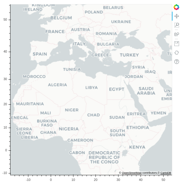
In [29]:
import matplotlib.pyplot as plt
gdf.plot()
Out[29]:

Folium Plots
In [5]:
gdf.head(1)
Out[5]:
In [6]:
# import the library
import folium
# Create a map with a center and zoom level
mapa = folium.Map(location= [-15.783333, -47.866667],
                  zoom_start= 1,
                  tiles= "OpenStreetMap")
mapa
Out[6]:
In [7]:
# Add the geodataframe as a geojson feature
points = folium.features.GeoJson(gdf,
                                 # tooltip with the name
                                tooltip=folium.GeoJsonTooltip(fields=['name']))
# Adding the feature to the canvas we created
mapa.add_child(points)
mapa
Out[7]:
Onward to Polygons
In [8]:
world = geopandas.read_file(geopandas.datasets.get_path('naturalearth_lowres'))
world.head(2)
Out[8]:
In [9]:
#https://matplotlib.org/3.1.1/gallery/color/colormap_reference.html
world.plot(figsize=(20,5), column= 'gdp_md_est', cmap='YlGnBu', legend=True)
Out[9]:

With Folium
In [10]:
import branca.colormap as cm
colormap = cm.linear.YlGnBu_09.to_step(data=world['gdp_md_est'], n=9)
colormap
Out[10]:
In [11]:
m = folium.Map()
# Setting the style
style_function = lambda x: {
    # How to fill color of the polygon
    'fillColor': colormap(x['properties']['gdp_md_est']),
    # Color of Polygon
    'color': 'black',
    # Weight of the border (Around the Polygon)
    'weight': 0.5,
    # Opacity of filled color
    'fillOpacity': 0.75
}
In [12]:
# Creating a geojson map with the style
folium.GeoJson(
    world,
    tooltip=folium.GeoJsonTooltip(fields= ["name", "gdp_md_est"]),
    style_function=style_function
).add_to(m)
# Add the legend to the same canvas
colormap.add_to(m)
m
Out[12]:
Marker Clusters
In [13]:
from folium.plugins import MarkerCluster
locations = []
# City location geometries to a list of latlongs pairs
for idx, row in gdf.iterrows():
    locations.append([row['geometry'].y, row['geometry'].x])
# Empty canvas
m = folium.Map()
# Markercluster
m.add_child(MarkerCluster(locations=locations))
m
Out[13]:
Heatmap
In [14]:
from folium.plugins import HeatMap
m = folium.Map()
m.add_child(HeatMap(locations, radius=15))
m
Out[14]:
Mo data Mo Problems

kepler.gl
Kepler.gl is a data-agnostic, high-performance web-based application for visual exploration of large-scale geolocation data sets. Built on top of Mapbox GL and deck.gl, kepler.gl can render millions of points representing thousands of trips and perform spatial aggregations on the fly.
Jupyter Notebook > 5.3
pip install keplergl
JupyterLab
jupyter labextension install @jupyter-widgets/jupyterlab-manager keplergl-jupyter
![]()
Kepler uses config to customize its maps
{
  "version": "v1",
  "config": {
    "visState": {
      "filters": [
        {
          "dataId": "earthquakes",
          "id": "vo18yorx",
        }
      ],
      "layers": [
        {
          "id": "hty62yd",
          "type": "point",
          "config": {
            "dataId": "earthquakes",
            "label": "Point",
            "color": [
              23,
              184,
              190
            ],
            "columns": {
              "lat": "Latitude",
              "lng": "Longitude",
              "altitude": null
            },
.....
The UX flow is composed of five layers

Filters, Timelines and other cool perks


Bokeh
In [30]:
from bokeh.io import output_notebook
from bokeh.plotting import figure, output_file, show
from bokeh.tile_providers import CARTODBPOSITRON, get_provider
output_notebook()
tile_provider = get_provider(CARTODBPOSITRON)
p = figure(x_range=(-2000000, 6000000), y_range=(-1000000, 7000000),
           x_axis_type="mercator", y_axis_type="mercator")
p.add_tile(tile_provider)
show(p)
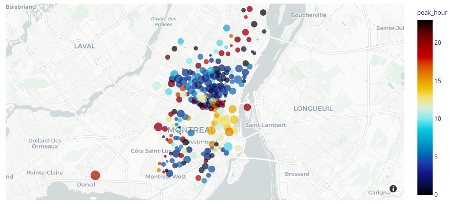
Plotly
In [16]:
import plotly.express as px
df = px.data.carshare()
fig = px.scatter_mapbox(df, lat="centroid_lat", lon="centroid_lon", color="peak_hour", size="car_hours",
                  color_continuous_scale=px.colors.cyclical.IceFire, size_max=15, zoom=10,
                  mapbox_style="carto-positron")
Say hello to Geopatra 👋
In [17]:
import geopatra
gdf.folium.plot(zoom=2)
Out[17]:
Yet another Library 😭
- this is not another library (Just a wrapper)
- An interface to interact with exisiting libraries without leaving the amazing geopandas ecosystem
- Netflix Syndrome
- I wanna be able to switch between them without having to remember all the interfaces/ spend time googling
Chloropeth maps
In [18]:
world.folium.chloropeth(color_by= 'pop_est',
          color= 'green',
          zoom= 1,
          style = {'color': 'black',
                    'weight': 1,
                    'dashArray': '10, 5',
                    'fillOpacity': 0.5,
                  })
Out[18]:
Circle Plots
In [19]:
gdf.folium.circle(radius=10, fill=True, fill_color='red', zoom=100, color='blue')
Out[19]:
Markercluster
In [20]:
gdf.folium.markercluster(zoom=1, tooltip=["name"])
Out[20]:
Weighted Markercluster
In [21]:
import random
gdf['value'] = [int(random.randint(10, 1000)) for i in range(len(gdf))]
gdf.folium.markercluster(zoom=1, metric='sum', weight='value')
Out[21]:
Heatmap
In [22]:
gdf.folium.heatmap(style={'min_opacity': 0.3}, zoom=5)
Out[22]:
Kepler.gl
In [24]:
from IPython.display import IFrame
kmap1 = gdf.kepler.plot()

Thank You : )
